45 pivot table concatenate row labels
How to Show Text in Pivot Table Values Area - Contextures Excel Tips There are special settings to use when you apply conditional formatting in a pivot table. To change the region numbers to text, follow these steps to manually add conditional formatting: Select all the Value cells in the pivot table (B5:F8). NOTE: B5 is the active cell, and you can see its address in the NameBox CONCATENATEX - DAX Guide Evaluates expression for each row on the table, then return the concatenation of those values in a single string result, seperated by the specified delimiter. Syntax CONCATENATEX ( , [, ] [, [, [] [, [, [] [, …
CONCATENATE EXCEPT BLANK VALUES - Power BI CONCATENATE EXCEPT BLANK VALUES. 08-17-2021 01:37 AM. I have the following code, in which I am creating a new column with the purpose of creating combinations of articles according to the sessionId. However, some of the 'Articles' rows are blank and therefore I would like to include in my code the condition to ignore the empty article rows and ...

Pivot table concatenate row labels
Concatenate rows using ids - Microsoft Power BI Community Hi @amitchandak, thanks for the quick response.Yes unfortunately it isn't the best data. It is sorted by roster period so the first set of dates is roster 1, second set is roster 2, etc. but they are all structured the same. Tutorial - How to Use a PivotTable to Create Custom Reports in ... 2. Create a pivot table. Select any cell in the source data table, and then go to the Insert tab > Tables group > PivotTable. This will open the Create PivotTable window. Make sure the correct table or range of cells is highlighted in the Table/Range field. Then choose the target location for your Excel pivot table: Excel Pivot Table tutorial - how to make and use ... - Ablebits Create a pivot table Select any cell in the source data table, and then go to the Insert tab > Tables group > PivotTable. This will open the Create PivotTable window. Make sure the correct table or range of cells is highlighted in the Table/Range field. Then choose the target location for your Excel pivot table:
Pivot table concatenate row labels. Show/Hide Field Headers in Excel Pivot Tables | MyExcelOnline Exercise Workbook: This is our pivot table. And you can see the 2 field headers on top: STEP 1: Go to PivotTable Analyze > Show > Field Headers. Click on it to hide the field headers: And they are now hidden! You can click on the same button to show them again. The headers will be visible again! Turn off automatic date and time grouping in Excel Pivot Tables Turn off date grouping in Excel Pivot Tables. You can turn off automatic date and time grouping in Excel Pivot Tables by changing the default behaviour in the Options settings. Click on your FILE menu item and choose Options. As shown below, in the DATA section choose to 'Disable automatic grouping of Date/ Time columns in Pivot Tables. Excel Consolidate Function - Guide to Combining Multiple Excel Files Step 3: On the Data ribbons, select Data Tools and then Consolidate. Step 4: Select the method of consolidation (in our example, it's Sum). Step 5: Select the data, including the labels, and click Add. Step 6: Repeat step 5 for each worksheet or workbook that contains the data you need included. Step 7: Check boxes "top row", "left ... PivotTable Text Values Alternative with FILTER - Excel University To create a list of the unique row labels (no duplicates), we would enter the following formula: =UNIQUE (Table1 [Client]) We hit Enter, and bam: If we wanted the row labels sorted, we could just wrap the SORT function around the UNIQUE function, like this: =SORT (UNIQUE (Table1 [Client])) And bam:
linkedin-skill-assessments-quizzes/microsoft-excel-quiz.md at main ... Q64. The PivotTable below has one row field and two column fields. How can you pivot this table to show the column fields as subtotals of each value in the row field? On the PivotTable itself, drag each Average field into the row fields area. Right-click a cell in the PivotTable and select PivotTable Options > Classic PivotTable layout. CONCATENATEX Values not showing up? - excelforum.com I have a pivot based on a very large dataset (800k rows) and there are some number values but also some text strings, so I use CONCATENATEX to convert those to text so I can include them in the pivot table. Sometimes when I create it then drag it to values, nothing happens. It processes then just nothing happens. Exploring Data with Excel Power Pivot - GeeksforGeeks Open one more clear activity manual in Excel. Click the PowerPivot tab on the Ribbon. Click Manage in the Data Model gathering. The Power Pivot window shows up. In the Power Pivot window, click the Home tab. Click From Database in the Get External Data bunch. Select From Database from the dropdown list. Custom Chart Data Labels In Excel With Formulas - How To Excel At Excel Follow the steps below to create the custom data labels. Select the chart label you want to change. In the formula-bar hit = (equals), select the cell reference containing your chart label's data. In this case, the first label is in cell E2. Finally, repeat for all your chart laebls.
pandas - How can I combine two different data frames into a pivot table ... What i'd like to do is put them side by side, and add two additional columns that subtract the difference by month of the new minus old, and then calculate the percentage change. The two tables are based on two data frames, df and hdf. Here is what the tables look like (old table that is, the new just includes 202003): Pivot columns - Power Query | Microsoft Docs To pivot a column. Select the column that you want to pivot. On the Transform tab in the Any column group, select Pivot column. In the Pivot column dialog box, in the Value column list, select Value. By default, Power Query will try to do a sum as the aggregation, but you can select the Advanced option to see other available aggregations. How to combine data in separate columns into a single row? Sep 28 2021 07:06 PM. Re: How to combine data in separate columns into a single row? do a power query on the data (left image) make 2 copies of the query using duplicate not reference, the first duplicate query you keep the value to the left, the 2nd duplicate you keep the value to the right. do a merge query matching the first column. Dynamic Chart Title by Linking and Reference to Cell in Excel Linking Cell to make Dynamic Chart Title - Step 2: Enter Cell Reference using Address bar. Go to the Address bar and type "=" and select a Cell to link. In the following example, we are linking the Cell D2. Dynamic chart title- Entering Cell Reference.
Informatica Scenarios:Pivoting of records(Pivoting of Employees by Department)
How do I filter a filter in a PivotTable? - Profit claims Example #1 Creating Inbuilt Filter in PIVOT Table Step 1: Lets have the data in one of the worksheets. The above data consists of 4 different columns with Sl.No, Flat Nos, Carpet Area & SBA. Step 2: Go to the Insert tab and select the Pivot table as shown below. When you click the pivot table, the Create Pivot Table window pops out.

Excel Pivot Table Combine Columns | Decoration Items Image
Create a Dynamic PivotTable Style Report with One Formula Starting with the header row, we combine the report labels ItemNum and Amount like this: =HSTACK ("ItemNum", "Amount") Moving into the body of the report, we populate the report label column using the SORT and UNIQUE functions. These will sort the unique values found in the ItemNum column of our data table. =SORT (UNIQUE (tbl_data [ItemNum]))
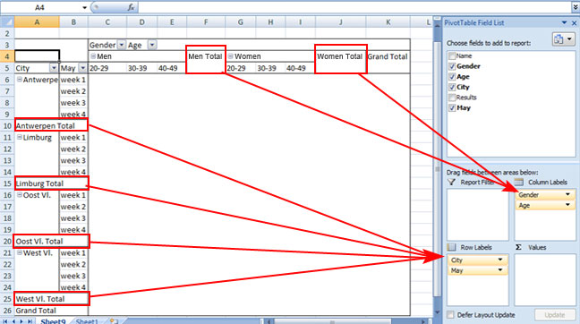
Lesson 55: Pivot Table Column Labels - Swotster
CONCATENATE function (DAX) - DAX | Microsoft Docs = CONCATENATE( [FirstName]&" ", CONCATENATE( IF( LEN([MiddleName])>1, LEFT([MiddleName],1)&" ", ""), [LastName])) This formula uses nested CONCATENATE and IF functions, together with the ampersand (&) operator, to conditionally concatenate three string values and add spaces as separators. Example: Concatenation of columns with different data types

How to Sort Pivot Table Row Labels, Column Field Labels and Data Values with Excel VBA Macro ...
How to Merge Duplicate Rows in Excel (3 Effective Methods) In the Tables group, select the PivotTable option. 3. The Create PivotTable dialog box will open up. Look at the Select a table or range field and look carefully if the selected range is correct. Choose Existing Worksheet. 4. Click on the Location icon and select the location (Here in Cell E4) where you want to place the resulting PivotTable.

get a row label from pivot table - Microsoft Tech Community
How to combine multiple rows into one column with pandas? Since I want to ignore the time point numbers and only want the twelve labels next to each other, pivot tables doesn't seem to do the job. python pandas. Share. Improve this question. Follow ... How to drop rows of Pandas DataFrame whose value in a certain column is NaN. 1298. Change column type in pandas. 3497. How to iterate over rows in a ...

Pivot table row labels in separate columns • AuditExcel.co.za
Macro to Concatenate Multiple Columns in Excel (with UDF ... - ExcelDemy Select the column where you want to concatenate the range and enter this formula: =ConcatenateColumns (B4:D14, {1,3},", ") Here we'll concatenate columns 1 and 3 of the data set B4:D14 ( Employee Name and Salary ). You use your one. Then press CTRL + SHIFT + ENTER ( Array Formula ).

Informatica Scenarios:Pivoting of records(Pivoting of Employees by Department)
How to Create Pivot Tables in R? - GeeksforGeeks Syntax: df %>% group_by ( grouping_variables) %>% summarize ( label = aggregate_fun () ) Parameter: df: determines the data frame in use. grouping_variables: determine the variable used to group data. aggregate_fun (): determines the function used for summary. for example, sum, mean, etc. Example 1: Create pivot tables R

Pivot Table Excel 2007 Repeat Row Labels | Elcho Table
How to Expand and Collapse Pivot Table Fields Levels In the Row Labels area: Right-click on one of the headings in the outermost field, click Expand/Collapse, then click click Expand Entire Field or Collapse Entire Field. Right-click on one of the headings in the outermost field, click Expand/Collapse, then click click Expand To or Collapse To, for the lowest level field.
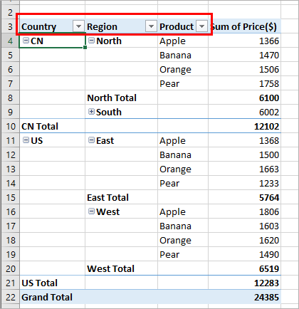
How To Create A Pivot Table With Multiple Columns And Rows | Cabinets Matttroy
Merge two relational data sets - Get Digital Help Select all cells you want to convert to an Excel Table. Press CTRL + T to create an Excel Table, a dialog box is displayed. Enable the checkbox if the Table has headers. Press with left mouse button on OK button. Excel applies automatically cell formatting to a new Excel Table, you can change the Table style if you don't like it.
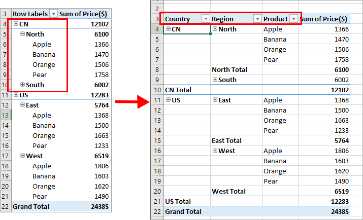
How To Create A Pivot Table With Multiple Columns And Rows | Cabinets Matttroy
Pivot table for non-numerical values using Pandas Recently I got the requirement to create pivot table for text values to be aggregated and concatenated with ',' for same row label in pandas. It can be easily done using crosstab tool in Alteryx. We'll be doing that using pandas for the quick tutorial. Data The data is the feedback survey form and exported as something like below table.
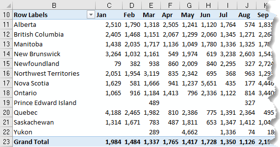
GETPIVOTDATA Function for Power Pivot • My Online Training Hub
TEXTJOIN function in Excel to merge text from multiple cells - Ablebits =CONCATENATE (A2, ", ", B2, ", ", C2) With Excel TEXTJOIN, you specify the delimiter just once in the first argument, and supply a range of cells for the third argument: =TEXTJOIN (", ", TRUE, A2:C2) TEXTJOIN in Excel - 6 things to remember To effectively use TEXTJOIN in your worksheets, there are a few important points to take notice of:

Excel Vba Sheet Name ändern - Extract the first middle and last name in Excel 2010 Microsoft VBA ...
Search table for each type of Service and concatenate the corresponding ... Then I looked into Filter and Index and Match and various other formulas but couldn't quite get it to come together. Here are two formulas I used that yielded results, but they are only part of the formula, I know: Concatenate: =TEXTJOIN (". ",TRUE, (2022H [Notes])) Identify the unique service: =UNIQUE (2022H [Service]) I don't know VBA.

How to Sort Pivot Table Row Labels, Column Field Labels and Data Values with Excel VBA Macro ...
Excel Pivot Table tutorial - how to make and use ... - Ablebits Create a pivot table Select any cell in the source data table, and then go to the Insert tab > Tables group > PivotTable. This will open the Create PivotTable window. Make sure the correct table or range of cells is highlighted in the Table/Range field. Then choose the target location for your Excel pivot table:
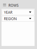
Insert Subtotals to a Pivot Table | MyExcelOnline
Tutorial - How to Use a PivotTable to Create Custom Reports in ... 2. Create a pivot table. Select any cell in the source data table, and then go to the Insert tab > Tables group > PivotTable. This will open the Create PivotTable window. Make sure the correct table or range of cells is highlighted in the Table/Range field. Then choose the target location for your Excel pivot table:

Excel: Show Customer Account & Name - Excel Articles
Concatenate rows using ids - Microsoft Power BI Community Hi @amitchandak, thanks for the quick response.Yes unfortunately it isn't the best data. It is sorted by roster period so the first set of dates is roster 1, second set is roster 2, etc. but they are all structured the same.
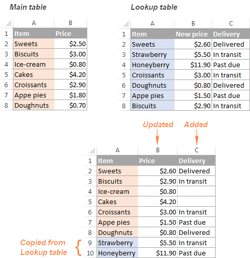
Consolidate in Excel: Merge multiple sheets into one
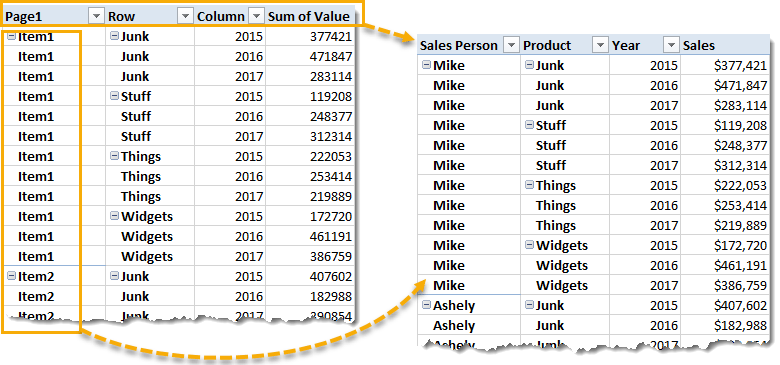
Excel Pivot Table Combine Columns | Decoration Items Image

Repeat Pivot Table row labels • AuditExcel.co.za Pivot Tables Course
Post a Comment for "45 pivot table concatenate row labels"